The TV-regularized stereo disparity implementation in this repo is based on the following paper:
Pock, Thomas, et al. "A convex formulation of continuous multi-label problems." Computer Vision–ECCV 2008: 10th European Conference on Computer Vision, Marseille, France, October 12-18, 2008, Proceedings, Part III 10. Springer Berlin Heidelberg, 2008.
Inputs:
Image Left
Image right
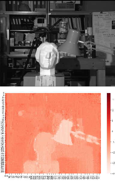
Output results:
Duality gap
Output disparity
Version
cmake
3.22
Python
3.8.10
OpenCV
4.5.1
libtbb-dev
2020.1-2
OpenMP
4.5
How to build and run
$ git clone https://github.com/raymondngiam/tv-regularized-stereo-disparity-in-opencv.git
$ cd tv-regularized-stereo-disparity-in-opencv
$ mkdir build && cd build
$ cmake ..
$ make
$ make install
$ cd .. /install/bin/release/
$ ./main
Let u ( x , y ) u(x,y) u ( x , y ) I 1 ( x , y ) I_1(x,y) I 1 ( x , y ) I 2 ( x , y ) I_2(x,y) I 2 ( x , y )
I 1 ( x , y ) = I 2 ( x + u ( x , y ) , y ) I_1(x,y) = I_2(x+u(x,y),y) I 1 ( x , y ) = I 2 ( x + u ( x , y ) , y )
From here onwards, we represent the input space as vector x = [ x y ] \mathbf{x} = \begin{bmatrix}x \\
y
\end{bmatrix} x = [ x y ]
Let ρ ( x , u ( x ) ) \rho(\mathbf{x},u(\mathbf{x})) ρ ( x , u ( x ))
ρ ( x , u ( x ) ) = ∣ I 1 ( [ x y ] ) − I 2 ( [ x + u ( x ) y ] ) ∣ \rho(\mathbf{x},u(\mathbf{x})) = |I_1(\begin{bmatrix}x \\
y
\end{bmatrix}) - I_2(\begin{bmatrix}x + u(\mathbf{x}) \\
y
\end{bmatrix})| ρ ( x , u ( x )) = ∣ I 1 ( [ x y ] ) − I 2 ( [ x + u ( x ) y ] ) ∣
The variational stereo disparity problem with total variation regularization is thus given by
min u { ∫ Ω ρ ( x , u ( x ) ) d x + λ ∫ Ω ∣ ∇ u ( x ) ∣ d x } (Eq. 1) \min_u \biggl\{ \int_{\Omega} \rho(\mathbf{x},u(\mathbf{x})) d\mathbf{x} + \lambda \int_{\Omega} |\nabla u(\mathbf{x})|d\mathbf{x}\biggr\}\space \space \text{(Eq. 1)} u min { ∫ Ω ρ ( x , u ( x )) d x + λ ∫ Ω ∣∇ u ( x ) ∣ d x } (Eq. 1)
where λ \lambda λ
The key idea is to lift the original problem formulation to a higher dimensional space by representing u u u
Let the characteristic function 1 u > γ ( x ) : Ω → { 0 , 1 } \mathbf{1}_{u>\gamma} (\mathbf{x}): \Omega \rightarrow \{0,1\} 1 u > γ ( x ) : Ω → { 0 , 1 } γ \gamma γ u u u
1 u > γ ( x ) = { 1 ,if u ( x ) > γ 0 otherwise. \mathbf{1}_{u>\gamma} (\mathbf{x}) = \Bigl\{ \begin{matrix} 1 & \text{,if }u(\mathbf{x})>\gamma\\
0 & \text{otherwise.}
\end{matrix} 1 u > γ ( x ) = { 1 0 ,if u ( x ) > γ otherwise.
Next, we make use of the above defined characteristic functions to construct a binary function ϕ \phi ϕ u u u
Let ϕ : [ Ω × Γ ] → { 0 , 1 } \phi : [\Omega \times \Gamma] \rightarrow \{0,1\} ϕ : [ Ω × Γ ] → { 0 , 1 }
ϕ ( x , γ ) = 1 u > γ ( x ) \phi(\mathbf{x},\gamma) = \mathbf{1}_{u>\gamma} (\mathbf{x}) ϕ ( x , γ ) = 1 u > γ ( x )
We can see that ϕ ( x , γ m i n ) = 1 \phi(x, \gamma_{min}) = 1 ϕ ( x , γ min ) = 1 ϕ ( x , γ m a x ) = 0 \phi(x, \gamma_{max}) = 0 ϕ ( x , γ ma x ) = 0 ϕ \phi ϕ
D ′ = { ϕ : [ Ω × Γ ] → { 0 , 1 } ∣ ϕ ( x , γ m i n ) = 1 , ϕ ( x , γ m a x ) = 0 } D' = \{ \phi : [\Omega \times \Gamma] \rightarrow \{0,1\} \space | \space \phi(x, \gamma_{min}) = 1, \phi(x, \gamma_{max}) = 0 \} D ′ = { ϕ : [ Ω × Γ ] → { 0 , 1 } ∣ ϕ ( x , γ min ) = 1 , ϕ ( x , γ ma x ) = 0 }
Note that the function u u u ϕ \phi ϕ
u ( x ) = γ m i n + ∫ Γ ϕ ( x , γ ) d γ u(\mathbf{x}) = \gamma_{min} + \int_{\Gamma} \phi(\mathbf{x},\gamma) d\gamma u ( x ) = γ min + ∫ Γ ϕ ( x , γ ) d γ
The previous variational stereo disparity problem in Eq.1 can be rewritten as,
min ϕ ∈ D ′ { ∫ Ω ∫ Γ ρ ( x , u ( x ) ) ∣ ∂ γ ϕ ( x , γ ) ∣ d γ d x + λ ∫ Γ ∫ Ω ∣ ∇ x ϕ ( x , γ ) ∣ d x d γ } \min_{\phi \in D'} \biggl\{ \int_{\Omega}\int_{\Gamma} \rho(\mathbf{x},u(\mathbf{x})) |\partial_\gamma \phi(\mathbf{x},\gamma)| \space d\gamma d\mathbf{x} + \lambda \int_{\Gamma}\int_{\Omega} |\nabla_{\mathbf{x}} \phi(\mathbf{x},\gamma)|\space d\mathbf{x} d\gamma \biggr\} ϕ ∈ D ′ min { ∫ Ω ∫ Γ ρ ( x , u ( x )) ∣ ∂ γ ϕ ( x , γ ) ∣ d γ d x + λ ∫ Γ ∫ Ω ∣ ∇ x ϕ ( x , γ ) ∣ d x d γ }
min ϕ ∈ D ′ { ∫ Ω ∫ Γ { ρ ( x , u ( x ) ) ∣ ∂ γ ϕ ( x , γ ) ∣ + λ ∣ ∇ x ϕ ( x , γ ) ∣ } d x d γ } (Eq. 2) \min_{\phi \in D'} \biggl\{ \int_{\Omega}\int_{\Gamma} \biggl\{\rho(\mathbf{x},u(\mathbf{x})) |\partial_\gamma \phi(\mathbf{x},\gamma)| \space + \lambda |\nabla_{\mathbf{x}} \phi(\mathbf{x},\gamma)| \biggr\}\space d\mathbf{x} d\gamma \biggr\} \space \space \text{(Eq. 2)} ϕ ∈ D ′ min { ∫ Ω ∫ Γ { ρ ( x , u ( x )) ∣ ∂ γ ϕ ( x , γ ) ∣ + λ ∣ ∇ x ϕ ( x , γ ) ∣ } d x d γ } (Eq. 2)
The second part (or smoothness term) of the equation above is based on the co-area formula, which essentially states that the TV norm can be decomposed into a sum of the length of the level sets of u u u
Although the current formulation is convex in ϕ \phi ϕ D ′ D' D ′
The idea is now to relax the variational problem by allowing ϕ \phi ϕ [ 0 , 1 ] [0, 1] [ 0 , 1 ] ϕ \phi ϕ
D = { ϕ : [ Ω × Γ ] → [ 0 , 1 ] ∣ ϕ ( x , γ m i n ) = 1 , ϕ ( x , γ m a x ) = 0 } D = \{\phi : [\Omega \times \Gamma] \rightarrow [0,1] \space | \space \phi(\mathbf{x}, \gamma_{min}) = 1, \phi(\mathbf{x}, \gamma_{max}) = 0 \} D = { ϕ : [ Ω × Γ ] → [ 0 , 1 ] ∣ ϕ ( x , γ min ) = 1 , ϕ ( x , γ ma x ) = 0 }
Hence the associated variational problem is now,
min ϕ ∈ D { ∫ Ω ∫ Γ { ρ ( x , u ( x ) ) ∣ ∂ γ ϕ ( x , γ ) ∣ + λ ∣ ∇ x ϕ ( x , γ ) ∣ } d x d γ } (Eq. 3) \min_{\phi \in D} \biggl\{ \int_{\Omega}\int_{\Gamma} \biggl\{\rho(\mathbf{x},u(\mathbf{x})) |\partial_\gamma \phi(\mathbf{x},\gamma)| \space + \lambda |\nabla_{\mathbf{x}} \phi(\mathbf{x},\gamma)| \biggr\}\space d\mathbf{x} d\gamma \biggr\} \space \space \text{(Eq. 3)} ϕ ∈ D min { ∫ Ω ∫ Γ { ρ ( x , u ( x )) ∣ ∂ γ ϕ ( x , γ ) ∣ + λ ∣ ∇ x ϕ ( x , γ ) ∣ } d x d γ } (Eq. 3)
The fundamental approach to minimize Eq. 3 is to solve its associated Euler-Lagrange differential equation.
E ( ϕ , ϕ ′ ) = ∫ L ( ϕ , ϕ ′ ) d x E(\phi,\phi')=\int \mathcal{L}(\phi,\phi')dx E ( ϕ , ϕ ′ ) = ∫ L ( ϕ , ϕ ′ ) d x
L ( ϕ , ϕ ′ ) = ρ ( x , u ( x ) ) ∣ ∂ γ ϕ ( x , γ ) ∣ + λ ∣ ∇ x ϕ ( x , γ ) ∣ \mathcal{L}(\phi,\phi') = \rho(\mathbf{x},u(\mathbf{x})) |\partial_\gamma \phi(\mathbf{x},\gamma)| \space + \lambda |\nabla_{\mathbf{x}} \phi(\mathbf{x},\gamma)| L ( ϕ , ϕ ′ ) = ρ ( x , u ( x )) ∣ ∂ γ ϕ ( x , γ ) ∣ + λ ∣ ∇ x ϕ ( x , γ ) ∣
d E d ϕ = ∂ L ∂ ϕ − div ∂ L ∂ ϕ ′ \frac{dE}{d\phi} = \frac{\partial \mathcal{L}}{\partial \phi} - \text{div}\frac{\partial \mathcal{L}}{\partial \phi'} d ϕ d E = ∂ ϕ ∂ L − div ∂ ϕ ′ ∂ L
d E d ϕ = − ∂ γ ( ρ ( x , u ( x ) ) ∂ γ ϕ ( x , γ ) ∣ ∂ γ ϕ ( x , γ ) ∣ ) − λ div ∇ x ϕ ( x , γ ) ∣ ∇ x ϕ ( x , γ ) ∣ \frac{dE}{d\phi} = -\partial_\gamma (\rho(\mathbf{x},u(\mathbf{x}))\frac{\partial_\gamma \phi(\mathbf{x},\gamma)}{|\partial_\gamma \phi(\mathbf{x},\gamma)|}) - \lambda \space \text{div}\frac{\nabla_{\mathbf{x}} \phi(\mathbf{x},\gamma)}{|\nabla_{\mathbf{x}} \phi(\mathbf{x},\gamma)|} d ϕ d E = − ∂ γ ( ρ ( x , u ( x )) ∣ ∂ γ ϕ ( x , γ ) ∣ ∂ γ ϕ ( x , γ ) ) − λ div ∣ ∇ x ϕ ( x , γ ) ∣ ∇ x ϕ ( x , γ )
It is easy to see that these equations are not defined either as ∣ ∇ x ϕ ( x , γ ) ∣ → 0 |\nabla_{\mathbf{x}} \phi(\mathbf{x},\gamma)| \rightarrow 0 ∣ ∇ x ϕ ( x , γ ) ∣ → 0 ∣ ∂ γ ϕ ( x , γ ) ∣ → 0 |\partial_\gamma \phi(\mathbf{x},\gamma)| \rightarrow 0 ∣ ∂ γ ϕ ( x , γ ) ∣ → 0
In order to resolve these discontinuities, one could use regularized variants of these terms, e.g. ∣ ∇ x ϕ ( x , γ ) ∣ ϵ = ∣ ∇ x ϕ ( x , γ ) ∣ 2 + ϵ 2 |\nabla_{\mathbf{x}} \phi(\mathbf{x},\gamma)|_\epsilon = \sqrt{|\nabla_{\mathbf{x}} \phi(\mathbf{x},\gamma)|^2 + \epsilon^2} ∣ ∇ x ϕ ( x , γ ) ∣ ϵ = ∣ ∇ x ϕ ( x , γ ) ∣ 2 + ϵ 2 ∣ ∂ γ ϕ ( x , γ ) ∣ ϵ = ∣ ∂ γ ϕ ( x , γ ) ∣ 2 + ϵ 2 |\partial_\gamma \phi(\mathbf{x},\gamma)|_\epsilon = \sqrt{|\partial_\gamma \phi(\mathbf{x},\gamma)|^2 + \epsilon^2} ∣ ∂ γ ϕ ( x , γ ) ∣ ϵ = ∣ ∂ γ ϕ ( x , γ ) ∣ 2 + ϵ 2 ϵ \epsilon ϵ ϵ \epsilon ϵ
To overcome the non-differentiability of the term ρ ( x , u ( x ) ) ∣ ∂ γ ϕ ( x , γ ) ∣ + ∣ ∇ x ϕ ( x , γ ) ∣ \rho(\mathbf{x},u(\mathbf{x}))|\partial_\gamma \phi(\mathbf{x},\gamma)|+|\nabla_{\mathbf{x}} \phi(\mathbf{x},\gamma)| ρ ( x , u ( x )) ∣ ∂ γ ϕ ( x , γ ) ∣ + ∣ ∇ x ϕ ( x , γ ) ∣
ρ ( x , u ( x ) ) ∣ ∂ γ ϕ ( x , γ ) ∣ + λ ∣ ∇ x ϕ ( x , γ ) ∣ ≡ max p { p ⋅ ∇ 3 ϕ ( x , γ ) } s.t. p 1 2 + p 2 2 ≤ λ , ∣ p 3 ∣ ≤ ρ ( x , γ ) \rho(\mathbf{x},u(\mathbf{x}))|\partial_\gamma \phi(\mathbf{x},\gamma)|+ \lambda |\nabla_{\mathbf{x}} \phi(\mathbf{x},\gamma)| \equiv \max_{\mathbf{p}} \bigg\{\mathbf{p} \cdot \nabla_3 \phi(\mathbf{x},\gamma)\bigg\} \space \text{s.t.} \space \sqrt{p_1^2 + p_2^2} \leq \lambda , \space |p_3| \leq \ \rho(\mathbf{x},\gamma) ρ ( x , u ( x )) ∣ ∂ γ ϕ ( x , γ ) ∣ + λ ∣ ∇ x ϕ ( x , γ ) ∣ ≡ p max { p ⋅ ∇ 3 ϕ ( x , γ ) } s.t. p 1 2 + p 2 2 ≤ λ , ∣ p 3 ∣ ≤ ρ ( x , γ )
where p = ( p 1 , p 2 , p 3 ) T \mathbf{p} = (p_1, p_2, p_3)^T p = ( p 1 , p 2 , p 3 ) T ∇ 3 \nabla_3 ∇ 3
This, in turn, leads us to the following primal-dual formulation of the functional:
min ϕ ∈ D { max p ∈ C { ∫ Ω ∫ Γ p ⋅ ∇ 3 ϕ ( x , γ ) d γ d x } } \min_{\mathbf{\phi}\in D} \bigg\{\max_{\mathbf{p}\in C} \bigg\{\int_{\Omega}\int_{\Gamma} \mathbf{p}\cdot \nabla_3 \phi(\mathbf{x},\gamma)\space d\gamma d\mathbf{x}\bigg\}\bigg\} ϕ ∈ D min { p ∈ C max { ∫ Ω ∫ Γ p ⋅ ∇ 3 ϕ ( x , γ ) d γ d x } }
where
{ C : [ Ω × Γ ] → R 3 ∣ p 1 ( x , γ ) 2 + p 2 ( x , γ ) 2 ≤ λ , ∣ p 3 ( x , γ ) ∣ ≤ ρ ( x , γ ) } \{C : [\Omega \times \Gamma] \rightarrow \mathbb{R}^3 \space | \space \sqrt{p_1(\mathbf{x},\gamma)^2 + p_2(\mathbf{x},\gamma)^2} \leq \lambda, \space |p_3(\mathbf{x},\gamma)| \leq \rho(\mathbf{x},\gamma)\} { C : [ Ω × Γ ] → R 3 ∣ p 1 ( x , γ ) 2 + p 2 ( x , γ ) 2 ≤ λ , ∣ p 3 ( x , γ ) ∣ ≤ ρ ( x , γ )}
E ( ϕ , ϕ ′ , p , p ′ ) = ∫ L ( ϕ , ϕ ′ , p , p ′ ) d x E(\phi,\phi',\mathbf{p},\mathbf{p}')=\int \mathcal{L}(\phi,\phi',\mathbf{p},\mathbf{p}')dx E ( ϕ , ϕ ′ , p , p ′ ) = ∫ L ( ϕ , ϕ ′ , p , p ′ ) d x
L ( ϕ , ϕ ′ p , p ′ ) = p ( x , γ ) ⋅ ∇ 3 ϕ ( x , γ ) \mathcal{L}(\phi,\phi'\mathbf{p},\mathbf{p}') = \mathbf{p}(\mathbf{x},\gamma)\cdot\nabla_3 \phi(\mathbf{x},\gamma) L ( ϕ , ϕ ′ p , p ′ ) = p ( x , γ ) ⋅ ∇ 3 ϕ ( x , γ )
d E d ϕ = ∂ L ∂ ϕ − div ∂ L ∂ ϕ ′ \frac{dE}{d\phi} = \frac{\partial \mathcal{L}}{\partial \phi} - \text{div}\frac{\partial \mathcal{L}}{\partial \phi'} d ϕ d E = ∂ ϕ ∂ L − div ∂ ϕ ′ ∂ L
d E d ϕ = − div 3 p ( x , γ ) \frac{dE}{d\phi} = -\text{div}_3 \mathbf{p}(\mathbf{x},\gamma) d ϕ d E = − div 3 p ( x , γ )
d E d p = ∂ L ∂ p − div ∂ L ∂ p ′ \frac{dE}{d\mathbf{p}} = \frac{\partial \mathcal{L}}{\partial \mathbf{p}} - \text{div}\frac{\partial \mathcal{L}}{\partial \mathbf{p}'} d p d E = ∂ p ∂ L − div ∂ p ′ ∂ L
d E d p = ∇ 3 ϕ ( x , γ ) \frac{dE}{d\mathbf{p}} = \nabla_3 \phi(\mathbf{x},\gamma) d p d E = ∇ 3 ϕ ( x , γ )
Primal step: For fixed p \mathbf{p} p ϕ \phi ϕ ϕ k + 1 = ϕ k − ( − τ p d E d ϕ ) \phi^{k+1} = \phi^k - (-\tau_p \frac{dE}{d\phi}) ϕ k + 1 = ϕ k − ( − τ p d ϕ d E )
ϕ k + 1 ( x , γ ) = ϕ k ( x , γ ) + τ p div 3 p ( x , γ ) \phi^{k+1}(\mathbf{x},\gamma) = \phi^k(\mathbf{x},\gamma) + \tau_p \text{div}_3 \mathbf{p}(\mathbf{x},\gamma) ϕ k + 1 ( x , γ ) = ϕ k ( x , γ ) + τ p div 3 p ( x , γ )
Note, that the scheme does not ensure that ϕ k + 1 ∈ D \phi^{k+1} \in D ϕ k + 1 ∈ D ϕ k + 1 \phi^{k+1} ϕ k + 1 D D D P ϕ ( ϕ k + 1 ) \mathcal{P}_\phi(\phi^{k+1}) P ϕ ( ϕ k + 1 )
P ( ϕ k + 1 ) = { 0 , ϕ k + 1 ( x , γ ) < 0 1 , ϕ k + 1 ( x , γ ) > 1 ϕ k + 1 ( x , γ ) , otherwise \mathcal{P}(\phi^{k+1}) = \Bigg\{ \begin{matrix} 0 & \text{, }\phi^{k+1}(\mathbf{x},\gamma)< 0\\ 1 & \text{, }\phi^{k+1}(\mathbf{x},\gamma)> 1\\ \phi^{k+1}(\mathbf{x},\gamma) & \text{, otherwise}\end{matrix} P ( ϕ k + 1 ) = { 0 1 ϕ k + 1 ( x , γ ) , ϕ k + 1 ( x , γ ) < 0 , ϕ k + 1 ( x , γ ) > 1 , otherwise
Dual step: For fixed ϕ \phi ϕ p \mathbf{p} p
p k + 1 = p k + τ d d E d p \mathbf{p}^{k+1} = \mathbf{p}^k + \tau_d \frac{dE}{d\mathbf{p}} p k + 1 = p k + τ d d p d E
p k + 1 = p k + τ d ∇ 3 ϕ ( x , γ ) \mathbf{p}^{k+1} = \mathbf{p}^k + \tau_d \nabla_3 \phi(\mathbf{x},\gamma) p k + 1 = p k + τ d ∇ 3 ϕ ( x , γ )
Since we need to ensure that p k + 1 ∈ C \mathbf{p}^{k+1} \in C p k + 1 ∈ C p k + 1 \mathbf{p}^{k+1} p k + 1 C C C P p ( p k + 1 ) \mathcal{P}_\mathbf{p}(\mathbf{p}^{k+1}) P p ( p k + 1 )
P p ( p 1 k + 1 ) = p 1 k + 1 max ( 1 , p 1 2 + p 2 2 λ ) \mathcal{P}_\mathbf{p}(p_1^{k+1}) = \frac{p_1^{k+1}}{\text{max}(1,\frac{\sqrt{p_1^{2}+p_2^{2}}}{\lambda})} P p ( p 1 k + 1 ) = max ( 1 , λ p 1 2 + p 2 2 ) p 1 k + 1
P p ( p 2 k + 1 ) = p 2 k + 1 max ( 1 , p 1 2 + p 2 2 λ ) \mathcal{P}_\mathbf{p}(p_2^{k+1}) = \frac{p_2^{k+1}}{\text{max}(1,\frac{\sqrt{p_1^{2}+p_2^{2}}}{\lambda})} P p ( p 2 k + 1 ) = max ( 1 , λ p 1 2 + p 2 2 ) p 2 k + 1
P p ( p 3 k + 1 ) = p 3 k + 1 max ( 1 , ∣ p 3 ∣ ρ ) \mathcal{P}_\mathbf{p}(p_3^{k+1}) = \frac{p_3^{k+1}}{\text{max}(1,\frac{|p_3|}{\rho})} P p ( p 3 k + 1 ) = max ( 1 , ρ ∣ p 3 ∣ ) p 3 k + 1
From empirical observation, the algorithm converges as long as the product τ p τ d ≤ 1 3 \tau_p \tau_d \leq \frac{1}{3} τ p τ d ≤ 3 1 τ p = τ d = 1 3 \tau_p = \tau_d = \frac{1}{\sqrt{3}} τ p = τ d = 3 1
Pock, Thomas, et al. "A convex formulation of continuous multi-label problems." Computer Vision–ECCV 2008: 10th European Conference on Computer Vision, Marseille, France, October 12-18, 2008, Proceedings, Part III 10. Springer Berlin Heidelberg, 2008.